The agriculture in Catalonia (Spain) suffers from the excessive use of fertilization and the waste of irrigation water. Over-application of pig manure and flood irrigations can cause severe environmental damage. Thus, development of improved cultivation techniques, stricter controls, and gathering of more detailed information about the current crop state are necessary to solve these environmental problems. Recent developments in the agriculture tend to dose the amount of fertilizer according to the needs of the plants and the capacity of the soil. This has been made possible through a better understanding of complex mechanisms in the soil and their interactions with the plants. Besides, the remote sensing techniques have reached a development state which allows the derivation of important agricultural information with a reasonable temporal and spatial resolution in order to allow the control of the cultivation practice and to support the agriculturist decisions.
The goal is the development of a system based on hyperspectral remote sensing data which provides agricultural relevant information about the crop fields at a reasonable level of costs. The information will be offered to farmers or governmental institutions interested in the monitoring of the cultivation to improve the environmental conditions.
The paper is organized as follows: Chapter II describes the proposed method to derive agricultural relevant parameters from hyperspectral CASI data based on physical models. In Chapter III, the concept of data assimilation is explained in more detail. Chapter IV describes the measurement and flight campaigns, which took place at maize test sites in Catalonia. In chapter V, the results of calibration and validation of the proposed method and the crop growth models are described and discussed.
I. DERIVATION OF CROP PARAMETERS FROMHYPERSPECTRAL DATA
A. Radiative transfer models
The radiative transfer plays an important role in modern remote sensing techniques, as optical remote sensing sensors measure the earth surface reflected solar irradiation. For this project, we choose the ACRM canopy spectral model (A twolayer Canopy Reflectance Model) [5] for the calculation of the radiative transfer within vegetation canopies. It is based on the homogeneous multispectral model MSRM [6] and the SAIL model, which models the diffuse radiative transfer. The ACRM model accounts for non-lambertian soil reflectance, specular reflection of direct sun rays on leaves, the hot spot effect, a two-parameter leaf angle distribution and the spectral effect of cultivation rows. For the spectral properties of leaves, we choose the PROSPECT model [4].
B. Inverse problem
The derivation of crop parameters from hyperspectral remote sensing data can be regarded as an optimization problem, i.e. the goal is to search the set of crop and soil parameters, which are “best” suited to the observations. One possibility to solve this problem is to search the most probable set of parameters, which is the basis of the maximum likelihood methods. In our case, the goal is to find a set of unknown crop and soil parameters, for which the a posteriori probability of the parameters Vˆ with measured reflectances r* is maximal.
A basic problem is that the number of parameters describing the scene exceeds the number of the independent observations available. The reasons for this are the complexity of the vegetated earth surface and the influences on the measured reflectances. Therefore, it is impossible to find unique estimators only by relying on the measured reflectances, because the inverse function is ill-posed. A first step to solve this problem is to reduce the number of variable parameters, i.e. the input parameters of the physical models are divided in variable V and constant c.
C. Introduction of a priori information
The introduction of a priori information is another possibility to solve this ill-posed problem. In general, there are several possibilities to introduce a priori information into the inversion process due to the variety of available “knowledge”:
-
In-situ measurements of parameters at defined sites
-
Knowledge about parameters based on assumptions
-
Knowledge about the parameters’ range based on assumptions or measurements
To introduce this knowledge into the derivation process, we use a priori values V* and probabilities PVV and apply penalties p to maintain the parameters within the definition range. The final cost function C, which has to be minimized, is described in equation (1). It contains the difference between observed r* and physically modeled reflectances r=fACRM(V,c), the stochastic model for the observations Pbb, the a priori information, and the penalties p (see [2]).
C = (r* – r)Pbb (r* – r)+ … (V – V*)PVV (V – V*) + p (1)
The stochastic model for the a priori information PVV contains no covariances, and the variances are defined as a priori weights according to the definition range and the natural variability of each parameter. For example, the variance of the leaf area index (LAI) is defined as high as the whole definition range, because this parameter show high variability, whereas the specific leaf weight is supposed to remain constant within the fields and thus, the variance is defined as a fraction of the definition range. The a priori values themselves were set to in-situ measured values according to the specific hybrid or are set to standard values in case of parameters with high variability.
D. Model fitting
Due to the complexity of the physical models, an analytical minimization of C is not possible. Thus, the model inversion is conducted numerically using common mathematical methods. The following numerical optimization methods are applied: Simplex algorithm (Simulated annealing) SA, Quasi-Newton QN, and Levenberg-Marquardt LM.
II. ASSIMILATION OF DERIVED PARAMETERS INTO CROP GROWTH MODELS
For precision farming purposes, crop growth models are necessary, as the information derived only from remote sensing data is not sufficient for the agronomists. Remote sensing techniques provide information about the plant’s present state, but not about the growth and development processes. Therefore, the assimilation of remote sensing data into crop growth models could improve the prediction of later crop development. Besides, the use of crop growth models over large areas is limited by our ability to provide them with required input parameters. It is impossible to obtain area wide plant and soil characteristics directly from in-situ observations. Thus, remote sensing data are acquired to provide information about crop processes over large areas.
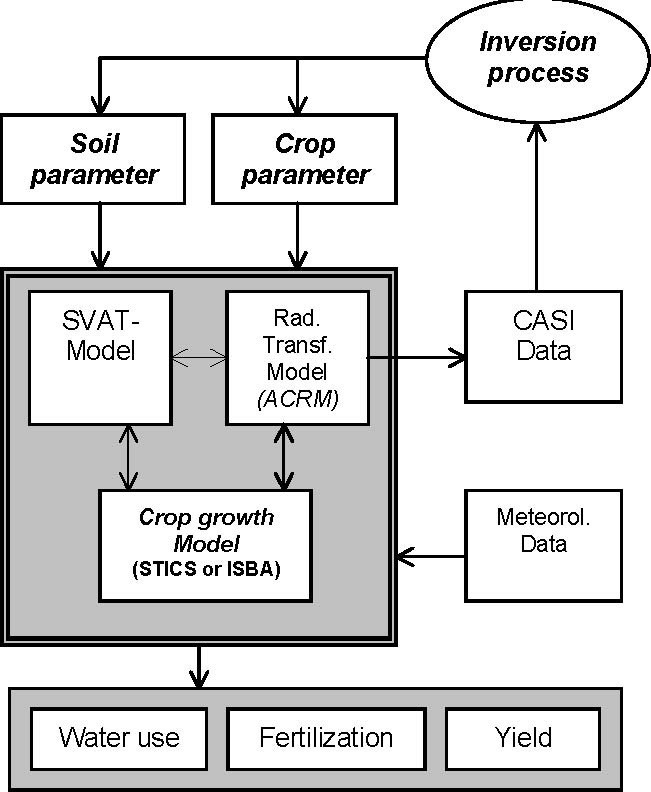
We select two crop growth models for the data assimilation, the STICS model [1] and the ISBA model [6] supported by simple SVAT (Soil Vegetation Atmosphere Transfer) models. Figure 1 gives an overview about the proposed assimilation of hyperspectral remote sensing data into the applied crop growth models. Crop and soil parameters are derived from the CASI reflectances using radiative transfer models like the ACRM model. Part of the derived parameters act as interface parameters, which are used to correct the continuous crop growth simulation of the STICS and ISBA models at the image acquisition dates. For this, various techniques can be applied: forcing (continuous), sequential assimilation (non continuous), and variational assimilation (adjustment). We propose a sequential assimilation of the derived parameters to improve the prognosis of water and fertilization use as well as crop yield.
First, we calibrate the STICS and ISBA models using in-situ measurements (not in this paper) to fit the hybrid and cultivation practices, then we validate the results of these models with non stressed crops (v. chapter V). Further investigations will be conducted to test the proposed data assimilation concept.

III. DATABASE
From May to August 2004, several measurement and flight campaigns were performed at six test sites near Lleida, Catalunya (0º57’ E, 41º40’ N). The test sites were planted with two different maize hybrids: Maize Oropesa and Maize Eleonora. In order to get different nitrogen amounts, selected parts of the test sites were left without nitrogen fertilization, whereas in the rest of the field nitrogen fertilization was applied. Simultaneously to the image acquisition dates, several cultivation, crop, and soil parameters were measured. Additionally, half-hour sampled meteorological parameters were obtained from the automatic weather stations.
A. Hyperspectral imagery
The CASI sensor was configured in the spatial mode with eleven spectral channels and a ground pixel size of about 10 meters. After the data acquisition, the hyperspectral images were calibrated and geometrically corrected. Then an atmospheric correction was done. For the physical atmosphere correction radiative transfer models based on the 6S code [8] were applied.
B. In-situ measurements
Simultaneously to the CASI image acquisition, crop and soil parameters were measured in-situ at all test sites taking into account the regions with different fertilization amounts. Thus, for each site and date, two plant and soil samples were taken and analyzed. Structural and chemical plant parameters were measured, the leaf area index, the leaf water content, nitrogen and chlorophyll content (SPAD readings), the specific leaf weight, soil water and nitrate content, etc. Besides, cultivation data (fertilization and irrigation date and amount, ploughing details, seeding date and density), constant soil parameters (soil structure, organic material, and soil chemical compounds), and selected meteorological data were recorded.
IV. RESULTS
The goal of the calibration process is to find optimal sets of configuration parameters for all applied models and inversion algorithms. Optimal configuration parameters are determined by comparing the RMSE of the derived parameters, the convergence, the amount of a priori information used, and the processing time. Table I compares the convergence and the processing time of model inversions for different configurations using synthetically generated CASI data. Best results are obtained by applying the LM algorithm with up to six variable parameters, which are selected according to the spectral sensitivity (sensitivity analysis not shown). In general, the introduction of a priori information improves the convergence and accuracy of the derived parameters, even in cases where the a priori information is slightly erroneous.
|
Experiment |
Inversion algorithm |
|||||||
|
Noise |
A priori info. |
Para-metes |
SA |
LM |
QN |
|||
|
No |
No |
5 |
99% |
6.5s |
99% |
0.5s |
96% |
1.5s |
|
No |
No |
6 |
94% |
10.0s |
98% |
1.0s |
91% |
1.5s |
|
No |
Yes |
6 |
99% |
10.0s |
99% |
1.0s |
99% |
1.5s |
|
Yes |
No |
5 |
65% |
10.5s |
75% |
1.0s |
72% |
1.5s |
|
Yes |
Yes |
5 |
99% |
10.5s |
93% |
1.0s |
99% |
1.5s |
| Yes | No | 6 | 45% | 20.0s | 53% | 1.6s | 59% | 2.5s |
| Yes | Yes | 6 | 97% | 20.0s | 99% | 1.6s | 99% | 2.5s |
| Yes | Yes | 13 | – | – | 73% | 3.0s | 78% | 6.6s |
In general, the above model and algorithm parameters are determined for the particular CASI configuration and the two maize hybrids Eleonora and Oropesa. For other configurations and hybrids, the calibration should be repeated.
|
Parameter |
A priori value |
A priori weight |
|
| Variable parameter |
Leaf area index |
1.0, 3.0a. |
0.25 |
| Leaf chlorophyll a content |
0.55 g/m2 |
0.25 |
|
| Leaf water content |
15.0 mg/cm2 |
0.25 |
|
| Leaf structure |
0.04, 0.01a. |
0.25 |
|
| Soil reflectance coefficients |
0.01 |
0.25 |
|
| Modal leaf angle |
60 |
1.0 |
|
| Eccentricity |
2.5 |
1.0 |
a. depending on the actual growth stage of the crop
B. Model validation
The model validation is conducted by comparing the in-situ measurements (meas), the derived parameters (CASI) and the simulations (STICS, ISBA) of the parameters LAI, dry matter (DM), leaf nitrogen (N), and leaf chlorophyll (Chl). Table III lists the linear regression coefficients. The comparisons of crop structure parameters LAI and dry matter show high correlation, whereas the derived chlorophyll values are not validated. The reasons for the bad correlation probably is bad georeferencing of the in-situ measurements, different scales (10m pixel vs. single leaves), and low accuracy in atmospheric correction of the CASI reflectances.
TABLE III. VALIDATION SUMMARY
|
LAISTICS |
LAIISBA |
LAICASI |
DMSTICS |
ChlCASI |
|
| LAImeas |
0.97b. |
0.99b. |
0.98 |
|
|
| LAICASI |
0.97b. |
0.87b. |
– |
||
| Dmmeas |
|
|
|
0.95 |
|
| Nmeas |
|
|
|
|
×a. |
| Chlmeas |
|
|
|
|
×a. |
a. ×: No significant correlation / b. Only test sites without nitrogen-or water stress
V. SUMMARY
A method to derive crop parameters from hyperspectral remote sensing data was designed, calibrated and validated with real measured data. For this, in-situ measurements and CASI imagery of test sites with two maize hybrids were acquired during six dates in 2004. The proposed derivation method showed good results in particular for crop structure parameters, LAI and the dry matter. Moreover, the inclusion of a priori information increased the convergence of the inversion process and accuracies of derived parameters.
A concept for the assimilation of remote sensing data into crop growth models was proposed. For this, two crop growth models were calibrated and validated using the in-situ measurements. Further investigations will be the sequential assimilation of the derived crop parameters to improve the model prediction of the crop growth models.
ACKNOWLEDGMENTS
The authors would like to thank Dr. Andres Kuusk affiliated with the Tartu Observatory in Tõravere Estonia and Dr. Jaan Praks affiliated with the University of Technology, Laboratory of Space Technology in Helsinki, for providing the code of the ACRM model including a module which deals with row structured vegetation surfaces, as well as Florence Habets affiliated with the Meteo-France Toulouse in France for providing the code of the ISBA crop growth model.