As a mapping agency in charge of most of the official cartographic production in Catalunya, ICC is flying every year in Catalonia an area of about 15 000 km2 at a ground sampling distance (GSD) of 45cm and an area of more than 500 km2 at a GSD of 7.5cm. Thus, a large database of analogue and digital images is available for a direct comparison between the analogue and the new digital workflow in terms of accuracy and efficiency.
During the validation process of the DMC at ICC some first conclusions about its performance were drawn (Alamus et al. 2005). Now, three years after the implementation of the digital cameras at ICC, the main part of the learning curve has passed, the workflows are well established and many production projects finished; therefore, it is time to study the performance of the new fully digital workflows in comparison to the old analog ones.
1. AERIAL TRIANGULATION
In aerial triangulation (AT) ICC’s in-house adjustment software ACX-GeoTex is used, which is able to employ highly precise GPS/INS observations for exterior orientation parameters, ground control observations and additional self-calibration parameters. For accuracy assessment two major differences between the analogue and the digital workflow must be considered: 1. The DMC has a smaller base to height (b/h) ratio of 0.3 (caused by the rectangular DMC image format) compared to the b/h ratio of 0.6 in the case of conventional analogue frame cameras, resulting in a two times lower accuracy estimation of the point heights. 2. In the analogue images nearly all measurements were stereoscopically observed by experienced operators on digital photogrammetric workstations, while from 2004 onward, almost at the same time the first digital DMC camera was purchased, this part was gradually taken over by automatic AT techniques using Inpho’s Match-AT software, i.e. most of the digital images were aerotriangulated using a dense photogrammetric network of automatically derived tie points. The automatic image correlation also returned a significant higher accuracy applied to digital images than applied to digitized analogue photos, which compensated a good part of the accuracy loss caused by the lower b/h ratio
1.1 Improvements in image pointing accuracy
During the validation of the first DMC camera in December 2004 manual and automatic aerotriangulations were performed and compared to the manual aerotriangulation of an analogue flight taken in 2000 from the same area (15mm scanning resolution).
The first topic to analyse is the point measurement accuracy applying semi-manual point identification in analogue and DMC images as well as digital image matching in the DMC images. Table 1 presents the pointing accuracy for semi-manual point identification in analog images, semi-manual point identification in DMC images (labeled DMC manual) and digital image matching (Match-AT) in DMC images. The table shows an improvement by a factor of 1.3 comparing the semi-manual point identification (point observation has been carried out using the semi-automatic tools provided by ISDM from Intergraph) of DMC and analogue images and even by a factor of 3 comparing digital image matching in DMC images to manual point identification in analogue images.
| Analog semiaut. | DMC semiaut. | DMC MatchAT | ||||
|
mm |
pix. |
mm |
pix. |
mm |
pix. |
|
| x |
4.83 |
0.32 |
2.85 |
0.24 |
1.23 |
0.10 |
| y |
4.27 |
0.29 |
2.35 |
0.20 |
1.12 |
0.09 |
Table 1: Photogrammetric residuals in mm and pixel (Alamús et al., 2005)
Image pointing accuracy using AAT techniques with analogue images is in the level of 4 to 5µm (i.e. 1/3rd of a pixel when scanned at 15µm), with DMC images it is in the level of 1.1 to 1.4µm (i.e. 1/10th of a pixel).
1.2 Small scale flights
To test the performance of aerial triangulation check points from several blocks have been analyzed. The analysis has been carried out in two different data sets: blocks with a GSD of 45cm, studied in this section and blocks with a GSD of 7.5cm, studied in the next section.
From year 2004 to 2007 ICC, in collaboration with the PNOA project, is flying and aerotriangulating half Catalonia at a GSD of 45cm, which corresponds to approximately 5000 DMC images every year. The check points used in the comparison were obtained from the 50 blocks used to aerotriangulate the 20 000 above mentioned images. It is important to point out that the used blocks are taken as they are without any kind of additional optimization. Therefore, the accuracies shown in the paper corresponds to a day to day work in a production environment rather than the result of an academic effort.
The accuracies of the check points shown in table 2 demonstrate that there is a slight improvement in the three coordinates when the DMC camera is used.
| RMS X (m) | RMS Y (m) | RMS H (m) | N.Checks | |
| Analog cameras | 0.22 | 0.20 | 0.28 | 90 |
| Digital (DMC) | 0.21 | 0.19 | 0.26 | 280 |
Table 2: Comparison of the analog vs. digital check point accuracies for 45cm GSD
In 2004 the ICC already had many years of experience in aerial triangulation of analog projects, but with the reception of the first DMC, in late 2004, some parts of the workflow had to be readjusted and some «know-how» had to be acquired (use of self calibration parameters, quality of GPS/IMU information, error propagation…) During the first 3 years of DMC operation an improvement on the quality of the aerial triangulations has been observed, which is attributed to the learning curve of the new technology. Fig. 1 shows the check point accuracy by year and a slight yearly improvement can easily be observed.

Fig. 1: Aerotriangulation check point accuracy vs. year of flight
The matching accuracy improvement observed in the correlation of digital images has not been translated to a big improvement in the horizontal accuracy because the check points are measured manually without any automatic or semiautomatic support. Concerning the small improvement in the vertical component, despite of the worse b/h factor, it has to be noticed that most of the check points are measured in images from different strips (flown at 25% side lap) so the «side lap b/h ratio» (when taking b as the base between images from different strips) plays an important role (and that value is similar in the analog and digital scenarios).
1.3 Large scale flights
Regarding the results from large scale flights, the check point accuracies from 25 different blocks are shown in table 3. The data corresponds to production urban projects with a GSD of 7.5cm for both digital and analog (scanned at 15mm) flights.
| RMS X (m) | RMS Y (m) | RMS H (m) | N.Checks | |
|
|
|
|
|
|
|
Digital (DMC) |
0.035 |
0.041 |
0.058 |
117 |
Table 3: Comparison of the analog vs. digital check point accuracies for 7.5cm GSD
For the combined horizontal accuracy, a very slight improvement in the digital flights can be observed while the vertical component of the accuracy remains stable. It has to be pointed out that the relative accuracy of the check points is at the level of 2cm, therefore it is possible that a portion of the residuals from the check points is due to the uncertainty of the ground coordinates.
As in the previous section the accuracy of the three components is very similar in analog and digital blocks. The explanation might be the same as in the previous section. The image observations of the check points are given by manual measurements (not taking advantage of the superior image correlation of the digital image) and in different strips (taking advantage of the side lap b/h ratio).
2. DEM GENERATION
This section describes and discusses the obtained accuracies of automatically DEMs derived for the same area from three different flight configurations The DEM are created using the commercial software package Match-T of the Inpho Company. The 3 flights were taken in a 3 year time difference with an analog RC30 camera at a ground pixel size of 45cm and with the DMC at a GSD of 45cm and 20cm. The major characteristics of the 3 corresponding blocks are listed in table 4.
|
Camera |
RC 30 |
DMC |
DMC |
| Year of flight |
2004 |
2006 |
2007 |
| Flying altitude [m] |
4700 |
4500 |
2000 |
| Focal length [mm] |
153 |
120 |
120 |
| GSD [cm] |
45 |
45 |
20 |
| Number of fotos |
136 |
326 |
234 |
|
Number of flight lines |
7 |
8 |
10 |
| End lap / side lap [%] |
60 / 25 |
60 / 25 |
60 / 25 |
Table 4: Block configurations
For the three blocks 3 DEMs were created with Match-T V5.0 setting the grid width approximately to the recommended value of 30 pixels; i.e. 15m for 45cm GSD and 7.5m for 20cm GSD. Low smoothing was chosen allowing the modeled surface to be close to the correlated point cloud. During the evaluation phase Match-T DSM V5.1 was released, which allows to further decrease grid width towards values of 10 pixels and below. With that version additional DEMs were created with a grid width of 10m and 5m for 45cm GSD and also 5m and 2m for 20cm GSD. For the comparison only «good» points were used, which were not classified by Match-T to have low redundancy or bad accuracy.
LIDAR data served as an independent reference, collected in January 2007 with an OPTECH ALTM 3025 system from 2 250m flying altitude. Parallel flight lines were flown with 20% side lap and a mean point density of 0.33 points/m2 in the non-overlapping areas. After ground classification this data is converted into a regular DTM with 2m grid width. Its accuracy is in the dm-level.
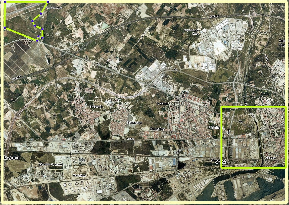
Test area was a 7.6km x 5.4km wide region close to the city of Tarragona in Spain (see fig. 2). It includes a 0.8km2 sized test-site in a flat area (TS_flat), which contains neither buildings nor higher vegetation and a 2.8km2 sized test-site in the city of Tarragona (TS_urban).
The grid points of the different versions were compared to the LIDAR data. The results are graphically represented in fig. 3. DEMs in different configuration were created for the entire test site (Match-T V5.0 only) and for the test sites TS_flat and TS_urban. The descriptors in fig. 3 indicate whether a digital (DMC) or an analog camera (RC30) was used, followed by the GSD in cm and the grid width deduced from that flight data. An appendix «_v51» is added if Match-T DSM V5.1 was used; e.g. «ana45_10m_v51» represents the results of a 10m spaced DEM obtained with Match-T DSM V5.1 from RC30 images having a ground pixel size of 45cm.
The DEM calculated for the entire test site as well as for TS_flat are compared to the regular spaced 2m DTM LIDAR data, representing the ground surface without vegetation and buildings. The DEM calculated for TS_urban is compared to the unclassified LIDAR point cloud representing also vegetation and buildings. The results for the three different test sites represent three different levels of accuracy. The represented standard deviations m are the results after filtering out all differences exceeding 3mIn case of test site TS_flat 1 2%, in the other cases an average of 15% of the differences was filtered out.

Figure 2: Test area (7.6 x 5.4 km2) with the two test-sites TS_flat (upper left) and TS_urban (lower right)

Figure 3: DEM accuracy
The most accurate results are obtained for test site TS_flat, where the DEM points are compared to the LIDAR DTM on a bare ground surface. In this flat area the DEM interpolation error is small and the comparison is more exact and reliable. Digital and analog images of 45cm ground pixel size result in more or less the same accuracy (1/2 ground pixel) with slight advantages for the DMC results. The digital images of 20cm GSD result in 8 to 9 cm accuracy reaching the accuracy level of the LIDAR data. The variation of the grid width has no significant impact on the results.
In test site TS_urban the DEM grid points are compared to the unclassified LIDAR points. Especially in urban areas the differences are much bigger, since the DEM grid points can not represent the height discontinuities at the edges of buildings or other man made objects. Fig. 4 shows a profile of the unclassified LIDAR points (white) and DEM grid points at 1m spacing derived from DMC images of 20cm GSD (red). The example shows, that some details resolved by LIDAR are not resolved by Match-T. For the 45cm pixels the accuracies obtained with analogue images are slightly better. The 10m and 5m spaced DEM, however, show big gaps where most of the points were classified to have low redundancy or bad accuracy. With DMC images a 10m and 5m spaced DEM from 45cm GSD could be derived without problems.

Figure 4: Differences between LIDAR points (white) and DEM grid points (red)
Finally a DEM of the entire testsite was calculated and compared to the regular 2m LIDAR DTM. Here standard deviations µ are achieved, which approximately correspond to the ground pixel size after filtering the differences which exceed 3µ (mostly points on buildings or high vegetation).
3. STEREOPLOTTING ACCURACY
As in the case of aerial triangulation the accuracy assessment of stereoplotting is done by comparing the coordinates of independent check points measured in the field with the coordinates of the same points observed in the stereo plotter.
3.1 Small scale flights
Stereoplotting of small scale flights, with 45cm GSD, is mainly used in the generation of the Topographic Database of Catalonia at 1:5.000 scale (BT-5M). The accuracy of this database, as indicated in the technical specifications, is 1m in the X and Y components and 1.5m in the H component in 90% of the points that can be well identified in stereo mode. The check points used are ground control points from the aerotriangulation of projects at larger scales but not used in the BT-5M aerotriangulation. The table 5 shows the results obtained in the comparison:
| RMS X (m) | RMS Y (m) | RMS H (m) | N.Checks | |
|
|
|
|
|
|
|
Digital (DMC) |
0.52 |
0.49 |
0.82 |
101 |
Table 5 Stereo plotting accuracy at independent check points for 45 cm GSD
As in the case of the aerial triangulation check points the horizontal accuracy is very similar in case of the analogical and digital images; however, in those cases, where the models are created along track, the worse b/h ratio leads to a small degradation of the vertical accuracy. It has to be pointed out, that even with that small degradation in height the BT-5M accuracy specifications for the project are fulfilled.
| 90% X (m) | 90% Y (m) | 90% height (m) | |
| Analog cameras |
0.80 |
0.83 |
1.17 |
| Digital (DMC) |
0.85 |
0.81 |
1.36 |
| BT-5M specification |
1.00 |
1.00 |
1.50 |
Table 6: Accuracy at 90% points for 45cm GSD
3.2 Large scale flights
Stereoplotting of large scale flights, with 7.5cm GSD, is mainly used in the generation of cartography of urban areas at 1:1.000 scale. The accuracy of this database, as indicated in the technical specifications is: 20cm in the X and Y components, and 25cm in H component in 90% of the points that can be well identified in stereo mode. The results obtained for the check points are shown in table 7:
| RMS X (m) | RMS Y (m) | RMS H (m) | N.Checks | |
|
|
|
|
|
|
|
Digital (DMC) |
0.087 |
0.091 |
0.103 |
29 |
able 7: Stereo plotting accuracy at independent check points for 7.5cm GSD
As in the smaller scale, the horizontal accuracy is very similar in case of the analogical and digital images and also a degradation of the vertical accuracy appears in the case of digital images. It has to be pointed that even with that small degradation in height the accuracy specifications for the project are fulfilled (see table 8). Notice that the vertical accuracy is only slightly worse than the horizontal accuracy in the digital images and even better than the horizontal accuracy in the analog image; we assume that this is due to the fact that the vertical component is determined from check points, which are part of an extended plane surface, represented in the image by more than 10 pixels: pavements, roofs, thick walls, etc.). Thus, during stereoplotting, the operator determines the height with the help of many pixels which implies a higher height accuracy potential compared to check points defined by one or just a few pixels only.
| 90% X (m) | 90% Y (m) | 90% height (m) | |
| Analog cameras |
0.173 |
0.160 |
0.102 |
| Digital (DMC) |
0.143 |
0.150 |
0.169 |
| BT-5M specification |
0.20 |
0.20 |
0.25 |
Table 8: Accuracy at 90% points for 7.5cm GSD
4. PHOTOINTERPRETATION
To analyze the photointerpretation changes derived of the stereoplotting process using images taken by the digital camera, only the opinions of well trained operators, with more than 5 years of experience using images taken by analogical cameras, has been taken into account. In the following a list of advantages and disadvantages is given in descending order of priority.
The first advantage is because the images contain more information in the shaded areas, more information can be displayed to be digitized. In the large scale flights to produce cartography at 1:1000 scale, the main consequence of having more information in shaded areas is that it has been possible to extend the flight period along the whole year, including winter, giving more flexibility to our production workflow. A second consequence, also in large scale flights where the digitized data is completed with field data to obtain cartography of urban areas, the digitization of more objects during the stereoplotting could reduce field data capture. Unfortunately no analysis has yet been done to know in detail the impact of this reduction, although that the estimated percentage will not achieve in any case more than 4 or 5%. In small scale flights it has not been possible to extend the flight period because the requirements in radiometry for orthophoto products require flights taken from May to September.
The second advantage is that usually the sharpness of the DMC images is higher than the obtained in the analogical ones at any scale, so the vector digitization is more comfortable for the operators.
The main disadvantage is a slight loss of the relief feeling. In large scale digital flights, with 7.5cm GSD, it is quite difficult to measure the height in objects lower than 20cm, like sidewalk curbstones or the rails of railways. These short measurements in height were possible using images taken by analogical cameras. This slight imprecision in the component H introduces some insecurity and uncomfortable feeling during the stereoplotting process.
Another disadvantage is the big differences in contrast between dark and bright areas. If the photogrammetric system doesn’t include some tools to modify more or less automatically the histogram during the stereoplotting process, the digitization process is harder than in the case of using analogical images where the contrast was not so high.
The last disadvantage is related to the reduction of the area covered by the digital stereopairs. It implies to manage twice as much files than in the case of analogical stereopairs and represents an extra cost during the stereoplotting process if the system hasn’t tools to change automatically to the adjacent stereopair.
5. IMAGE RESOLUTION
Traditionally, the resolving power of an optical system was measured by the visual identification of targets, amongst which the USAF 1951 test stood out due to the fact that it has been used more than others. With the same purpose electronic methods have been developed to assess the performance of a system, based on profiles of sinusoidal intensity and supported by the Modulation Transfer Function (MTF) and the Edge Spread Function (ESF). Our methodology is based on the latter.
A software tool is implemented with the aim of providing a resolving measurement of an image in pixel magnitude. The program processes a region of interest that contains a single contour and makes a minimum square adjustment over the bi-dimensional function of the edge that we model as a sigmoid function:
 (1)
(1)
The five parameters are estimated in a least squares adjustment and the computed function is derived for obtaining the LSF (Line Spread Function). We consider the FWHM (Full Width at Half Maximum) over the LSF to be the measurement value.
5.1 Results obtained with aerial images (DMC) and Siemens star targets
The algorithm has been applied on a Siemens star target painted on a canvas surface of 100m2 that has been captured in four DMC aerial images. The pattern used for this study can be seen on the top-right part of fig. 5. On each of the four images used for the test, the pattern was located at a different distance from the centre. The average resolution obtained for each image is shown in table 9.

Figure 5: Siemens star target used for the resolution study
|
Image |
Distance to the centre (pixel) |
Resolution (pixel) |
|
Image 1 |
1772 |
0.83 |
|
Image 2 |
1519 |
0.79 |
|
Image 3 |
4241 |
1.07 |
|
Image 4 |
4543 |
1.32 |
Table 9. Resolution measurements as function of the distance from the image centre
These results show that the distance to the centre of the image greatly affects the resolution. The main reason that explains this behaviour is the formation of the large format image from oblique component images. The 12μm size pixel gives us a nominal resolution of 84 l/mm. But, in fact, the resolution is not constant in the whole area of the large format virtual image. The sensor is tilted along the two axis x and y. This factor has been studied by Honkavaara et al. 2006 who obtained a resolution of 53 and 84 l/mm perpendicular to the direction of flight and around 60 and 84 l/mm in the direction of flight.
5.2 Results obtained with aerial images (DMC) on urban settings.
Finally, the aim is to apply concepts and techniques developed to images captured with DMC that do not have, necessarily, artificial models. Due to their radiometric and morphological characteristics (close to the USAF model) we chose to apply the software on images of urban settings. Adequate radiometric contours are considered to be road markings and, more precisely, pedestrian crossings, see fig. 6.

Figure 6: Pedestrian crossing
From each pedestrian crossing, a resolution measurement is extracted, taking the mean of several values obtained over different parts of the crossing, in order to minimise the effects of noise. Furthermore, frames with a high number of crossings, placed horizontally and vertically, have been chosen in order to compare the results that we obtain with the theoretical estimations that we already have.
The fig. 7 and 8 show the value of resolution obtained from the application of the software in different pedestrian crossings, based on the distance to the centre of the shot, compared to the theoretical values of resolution in flight and cross-flight direction, respectively.

Figure 7: Resolution cross-flight direction

Figure 8: Resolution flight direction
Conclusions
DMC digital images prove to have a big improvement in terms of image correlation reaching a matching accuracy of 1/10th of a pixel. In aerotriangulation check points showed that an accuracy of 1/2 pixel in the horizontal components and 2/3 of a pixel in the vertical component can be routinely archived in production flights. In this study, however, the high accuracy in the correlation of digital images is not reflected in the horizontal accuracy because the check points are measured manually without any automatic or semiautomatic support. Despite of the worse b/h factor a small improvement in the vertical accuracy has been observed. This is due to the fact that most of the check points are measured in images from different strips (flown at 25% side lap), where the (larger) “side lap b/h ratio” compensates the worse b/h in flight direction.
Automatically derived DEMs from digital and analog images result in more or less comparable accuracies with small advantages for the digital camera. Digital images also allow smaller grid spacing down to the size of 5 pixels. The comparison with LIDAR data proves a vertical accuracy of up to ½ pixels in flat areas without vegetation and buildings. In urban areas the accuracy is considerably worse (approximately 2 pixels), because the DEM grid points do not well represent the height discontinuities at the edges of buildings or other man made objects.
From the steroplotting point of view, the conclusion is that the use of digital images allows digitizing more information, extending the flight period and introducing more comfort in the steroplotting process. Although there is a slight loss of the relief feeling, and there is a small decrease in the height accuracy, it is not important enough to introduce degradations in the final products. Finally, more automatic tools are needed to optimize image display and management. Stereoplotting check points showed that an accuracy of 1.1 pixels in the horizontal components and about 1.5 pixels in the vertical component can also be routinely achieved in production projects.
Concerning the resolution of DMC digital images in the paper absolute resolution measures have been generated from a Siemens star target whose dimensions are known. The measurement FWHM which is extracted from the LSF function provides a specific quantification of the resolution of the system, coherent with techniques of resolution evaluation, using USAF targets. This very same methodology can also be applied to analogues images (Alamús et. al, 2005). The results then obtained, showed the greater resolution power of the DMC, in front of the film cameras.
References
Alamús, R., Kornus, W., Palà, V., Pérez, F., Arbiol, R., Bonet, R., Costa, J., Hernández, J., Marimon, J., Ortiz, M. À., Palma, E., Pla, M., Racero, S., Talaya, J. 2005: Validation process of the ICC digital camera. ISPRS Worshop “High-Resolution Earth Imaging for Geospatial Information”. Hannover.
Honkavaara, E., Jaakkola, J., Markelin, L., Becker, S., 2006. Evaluation of Resolving Power and MTF of DMC. In proceedings of ISPRS Comission I Symposium, Paris.
Acknowledgements: We would like to thank the hard job done by M. Cabré, J. Costa., J. Marimón and A. Serrano for the selection and measurement of the check points used in the aerial triangulation and stereoplotting accuracy assessment.